


I. Introduction

The human brain consists of a high percentage of water (around 77-78%), that scientists can gracefully detect/measure and finally give a better chance to a patient to extent his life and improve its quality, for example in the case of incurable brain diseases.
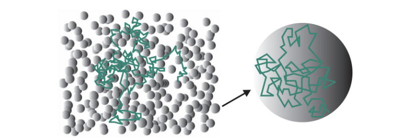
DW-MRI measures the signal of the proton (1H) in water molecules (H20), which corresponds to the movement of water molecules, by applying a set of magnetic gradient directions to the subject that we examine. This permits us to measure the motion of the molecules across these directions. This random movement is known as intra-voxel incoherent motion, random motion, or Brownian motion (rf. figure 2).
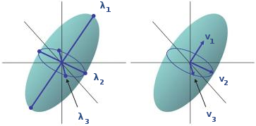
Diffusion models are tools that allow us to represent the diffusion of water molecules that captures the structure of the white matter of the brain. The first attempt took place with the introduction of Diffusion Tensor Imaging (DTI). DTI can only describe a single direction of diffusion in the underlying fiber architecture (rf. figures 3, 4(a)).
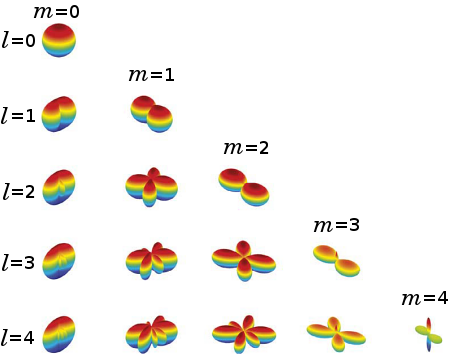
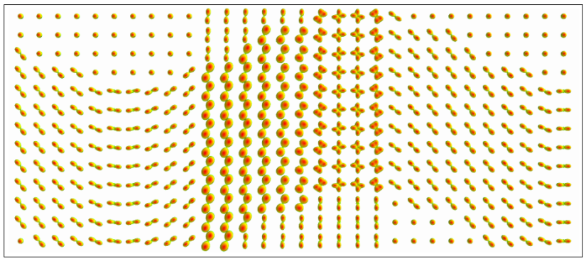
As neuro-scientists gained deep understanding of neuro-imaging, it was proved that more complex structures containing bundles of fibers can appear in the human brain (in almost 50% of the cases), meaning that more flexible models that can capture, in detail, the underlying shape of the fibers are required. In this direction, Higher Order Tensor (HOT) models became popular (rf. figures 4(b), 5).
II. High Level Description of DW-MRI Data
Until a few years ago, mapping the connection paths between different parts of the brain had only been possible via ex vivo invasive techniques, e.g. anatomical dissection, or in vivo chemical tracer methods. As a consequence, non-invasive techniques to monitor and study in vivo brain lesions, development etc. that will affect those networks were in great demand and well appreciated.
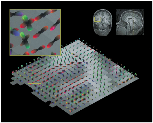
Fitting tensor models [1-4] to DW-MRI data permits us to approximate the underlying -fiber structure and to specify the main directions of diffusion (rf. figure 6, 7).
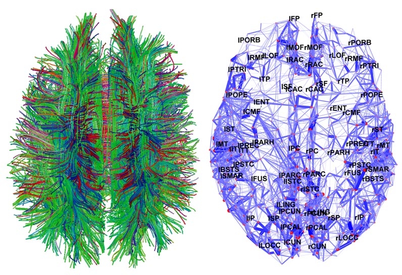
The strategy to determine connection paths of the brain which uses information derived from tensor models is known as tractography (rf. figures 8, 9).


FIGURE 8: Several examples of brain tractographies.

to adult and in-utero fetal brain studies. Medical Image Analysis, 17(3):297310., 2013.
III. Connectomes
From the beginning of neuroscience, understanding the functionality and the connectivity of neural elements of the brain and identifying anatomical units has puzzled and fascinated scientists (rf. figure 10). The evolution of science and the invention of different techniques, such as fMRI, EEG etc. or even tractographies, permit us to measure the activity of neurons and to localize their connections so that interesting relational paths between them can be depicted. As a consequence, the need of a proper way to model that information came to the foreground.
The answer to the problem of representing the connectivity was found with the aid of graph theory. The nodes of the networks represent neural units, while the edges reflect the associations between neural structures.
IV. DW-MRI Data Statistical Analysis
Generally in medical imaging, the term “atlas” (i.e. collection of maps) refers to an anatomical 3D representation of an area/organ (e.g. brain). An atlas is constructed by accumulating data of one or more subjects in a common coordinate system.
As the number of considered patients is increasing, statistical atlases (rf. figure 11) may be devised by extracting patterns characterizing a particular property/disease etc.. For example, these patterns can be calculated given a set of individual DW-MRI data that can be split into two groups, the normal population (or control group) and the abnormal population (or pathological or testing group) that contains patients of a specific disease (common between all abnormal individuals). Statistical atlases capture the variability of specific patterns in each population and are useful to determine biomarkers.

In the case where the number of individuals is large enough to completely capture the variability of both populations, then the project of constructing atlases related to a disease, by measuring the variability of the groups, is linked to the biomarker extraction problem. This is addressed through population versus population comparisons (rf. figures 12, 13).
FIGURE 12: Population VS population comparison in a voxel that DOESN’T contain any lesions (great SIMILARITY comparing the estimated distributions per population).
FIGURE 13: Population VS population comparison in a voxel that DOES contain many lesions (great DISSIMILARITY comparing the estimated distributions per population).
On the other hand, when the data are sparse (often happening in the case of the abnormal population) or when there is no common disease patterns between patients, it is hard (or meaningless) to construct the disease’s atlas, but it is possible to compare the state of each abnormal individual to the estimated distribution of the normal population via an individual versus normal population test.
FIGURE 14: Several examples of Individual VS Control population tests.
V. Population VS Population Comparison (fig. 12, 13): Application to NMO disease
Applying the proposed statistical approach within a region of interest for a specific disease can reveal an interesting list of p-values sorted in ascending order. It can highlight the most significantly different voxels (i.e. biomarkers) in the top of that list, which finally can help us to define regions of interest for each particular disease.
Extracting interesting biomarkers, or regions of them, that will signify that those specific regions are characteristic areas affected by the disease. In this way, we can provide useful information by guiding the doctors through their examination or to properly adjust the patient’s treatment.
VI. Individual VS Normal Population (fig. 14): Application to LIS disease
In cases where the variability of the abnormal population cannot be totally captured due to the lack of enough pathological data, it is not pertinent and even not safe to rely on population vs population approaches. The existence of empty (unlabeled) areas in the space, due to the lack of (abnormal) points, close to the mass of the normal population will result in data being probably misclassified as normal, in the absence of knowing completely the variability of the abnormal group.
Moreover, under certain circumstances, it is much more robust to evaluate the state of every patient separately, for example, in patient follow-up. As a consequence, each incoming abnormal dataset should be tested individually versus the normal population (in most of the cases is well-defined by a large dataset), which will permit us to follow the state of the patient across several in time scans in specific ROIs (rf. figure 15).
FIGURE 15: Performing patient’s follow up in three specific ROIs related to the studied brain disorder.Greyscale images referring to Franctional Anisotropy Images (FA images).
VII. Summary
To briefly conclude this post, what follows is a collective representation of what was previously presented above:
FIGURE 16
VIII. References
- Barmpoutis, A., Jian, B., Vemuri, B. C., and Shepherd, T. M. (2007). Symmetric positive 4th order tensors & their estimation from diffusion weighted MRI. In Proceedings of the Information Processing in Medical Imaging conference (IPMI), volume 4584 of Lecture Notes in Computer Science, pages 308-319. Springer.
-
Barmpoutis, A. and Vemuri, B. C. (2010). A unified framework for estimating diffusion tensors of any order with symmetric positive-definite constraints. In Proceedings of ISBI: IEEE International Symposium on Biomedical Imaging, pages 1385-1388.
- Weldeselassie, Y., Barmpoutis, A., and Atkins, S. (2012). Symmetric positive-definite Cartesian tensor fiber orientation distributions (CT-FOD). Medical Image Analysis, 16(6):1121-1129.
- Weldeselassie, Y. T., Barmpoutis, A., and Atkins, S. (2010). Symmetric positive-definite Cartesian tensor orientation distribution functions (CT-ODF). In International Conference on Medical Image Computing and Computer Assisted Intervention (MICCAI), volume 6361 of Lecture Notes in Computer Science, pages 582-589. Springer.
~ T.G. ~
If you are working in this scientific area, do not hesitate to contact me for any further question,
AND
do not forget to CITE our work! 😉
~ Paper in international conference ~
* T. Gkamas, F. Renard, C. Heinrich and S. Kremer, “A fourth order tensor statistical model for diffusion weighted MRI – application to population comparison“, International Conference on Pattern Recognition Applications and Methods (ICPRAM), Lisbon, Portugal, pages 277-282, January 2015.
~ Ph.D. Dissertation ~
Thesis’ Title: “Statistical Modelling of High Order Tensors in Diffusion Weighted Magnetic Resonance Imaging“, Doctoral School MSII 269, iCube-MIV group, University of Strasbourg, France, Sept. 2015.
~ Copyrights reserved by Gkamas et al.* and the University of Strasbourg. ~
MISC:
listening to a great Pink Floyd’s song talking about why it’s important to share our expertise for the grace of humanity, making it as the most valued decision to make in every scientist’s career:
![]() 🎶 ~ Pink Floyd – Talkin’ Hawkin’ ~ 🎶
🎶 ~ Pink Floyd – Talkin’ Hawkin’ ~ 🎶 ![]()
